It can be shown that this surface integral can be equivalently replaced by a line integral taken along the periphery of \(S\).
10.2 Line integral
The Stokes theorem states that, for any vector field \(\mathbf A = (A_x, 0, A_z)^\top\) there holds
\[
\int\limits_S (\nabla \times \mathbf A) \cdot d\mathbf s = \oint\limits_C \mathbf A \cdot d\mathbf \ell,
\]
where \(d\mathbf\ell = \mathbf e_x dx + \mathbf e_z dz\) is the oriented line element tangential to the curve \(C\), and \(d\mathbf s = dx \,dz \, \mathbf e_y\) the oriented surface element normal to the cross section \(S\). It follows by inspection that
\[
A_x = 0, \qquad A_z = -2 f \Delta\rho \, z \left(\frac{1}{z} \, \tan^{-1}\frac{x}{z}\right) = -2 f \Delta \rho \, \theta
\]
The angle \(\theta\) is taken from the positive \(x\)-axis towards the positive \(z\)-axis.
Talwani et al. (1959) have shown that the vertical component of the gravitational attraction of a two-dimensional prismatic body is, at the origin, equal to
\[
g_z(0, 0) = 2 f \Delta \rho \oint\limits_C z \, d\theta,
\]
i.e., a line integral taken along its periphery.
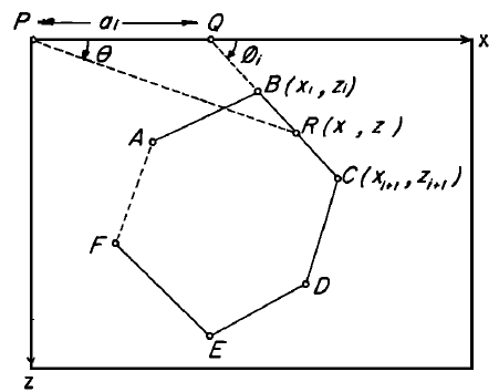
The following sketch illustrates the situation (taken from the original Talwani paper).
Let \(ABCDEF\) be a given polygon with \(n\) sides and let \(P\) be the point at which the gravitational attraction due to this body has to be computed.
Further, let \(z\) be defined positive downwards and let \(\theta\) be measured from the positive \(x\)-axis towards the positive \(z\)-axis.
Let us evaluate the integral \(\oint z\, d\theta\) for the above polygon.
We consider here the contribution from the side \(BC\). The remaining sides have to be added to obtain the total gravitational attraction of the complete prism.
At the point \(Q\) the line \(BC\) meets the \(x\)-axis at an angle \(\phi_i\).
Let \(PQ = a_i\). For any arbitrary point \(R = R(x,z)\) on the side \(BC\) there hold the two equivalent equations
\[
z = x \tan\theta
\]
and
\[
z = (x - a_i) \tan\phi_i.
\]
After eliminating \(x\) we obtain an expression for \(z = z(\theta)\):
\[
z = \frac{a_i \tan\phi_i \tan\theta}{\tan\phi_i - \tan\theta}
\]
The contribution of the segment \(BC\) to the above line integral can now be rewritten as
Note that with \[
\log\left( \frac{1}{\cos^2\theta}\right) = - 2 \log \cos\theta
\] and after combining the \(\log\) terms we obtain the desired integral taken in the limit of integration, i.e., \(\theta_i\) and \(\theta_{i+1}\), \[
Z_{i} =a_{i} \sin \phi_{i} \cos \phi_{i} \left[ \theta_{i}-\theta_{i+1} +\tan \phi_{i} \log _{e} \frac{\cos \theta_{i}\left(\tan \theta_{i}-\tan \phi_{i}\right)}{\cos \theta_{i+1}\left(\tan \theta_{i+1}-\tan \phi_{i}\right)}\right]
\] which is the equation for \(Z_i\) given in Talwani et al. (1959), p. 50.
Talwani, M., Worzel, J.L. & Landisman, M., 1959. Rapid gravity computations for two-dimensional bodies with application to the Mendocino submarine fracture zone. Journal of Geophysical Research, 64, 49–59. doi:10.1029/JZ064i001p00049
Zhou, X., 2008. 2D vector gravity potential and line integrals for the gravity anomaly caused by a 2D mass of depth-dependent density contrast. GEOPHYSICS, 73, I43–I50. doi:10.1190/1.2976116