11  Implementation of the TALWANI approach

We define a Python class Polygon which takes as argument a list of coordinates and a parameter. The purpose of this class is twofold:

Show the code
class Polygon:
    def __init__(self, x, z, density):
        xc = np.mean(x)
        zc = np.mean(z)
        angles = np.array([np.arctan2(p[1] - zc, p[0] - xc) for p in zip(x, z)])
        ind = np.argsort(angles) # if reverse order is required, flip sign of angles 
        x = x[ind]
        z = z[ind]
        x = np.append(x, x[0])
        z = np.append(z, z[0])
        x[isclose(x, 0.0)] = 0.0
        z[isclose(z, 0.0)] = 0.0
        self.x = x
        self.z = z
        self.density = density
        self.n = len(x) - 1

    def __str__(self):
        return f"n: {self.n} \nx:\n {self.x} \nz:\n {self.z} \nDensity:\n {self.density}"

To compare the numerical results, we provide here a simple function which computes the gravitational attraction of a horizontal cylinder of mass m that intersects the vertical plane at the coordinate given by the 2-D array axis. The point of observation is given by the coordinates in the 2-D array obs:

g = cylinder(obs, mass, axis)

Show the code
def cylinder(obs, mass, axis):
    g = -2 * 6.674e-11 * mass / np.linalg.norm(obs - axis)**2 * (obs - axis)
    return g

The following code implements the Talwani approach:
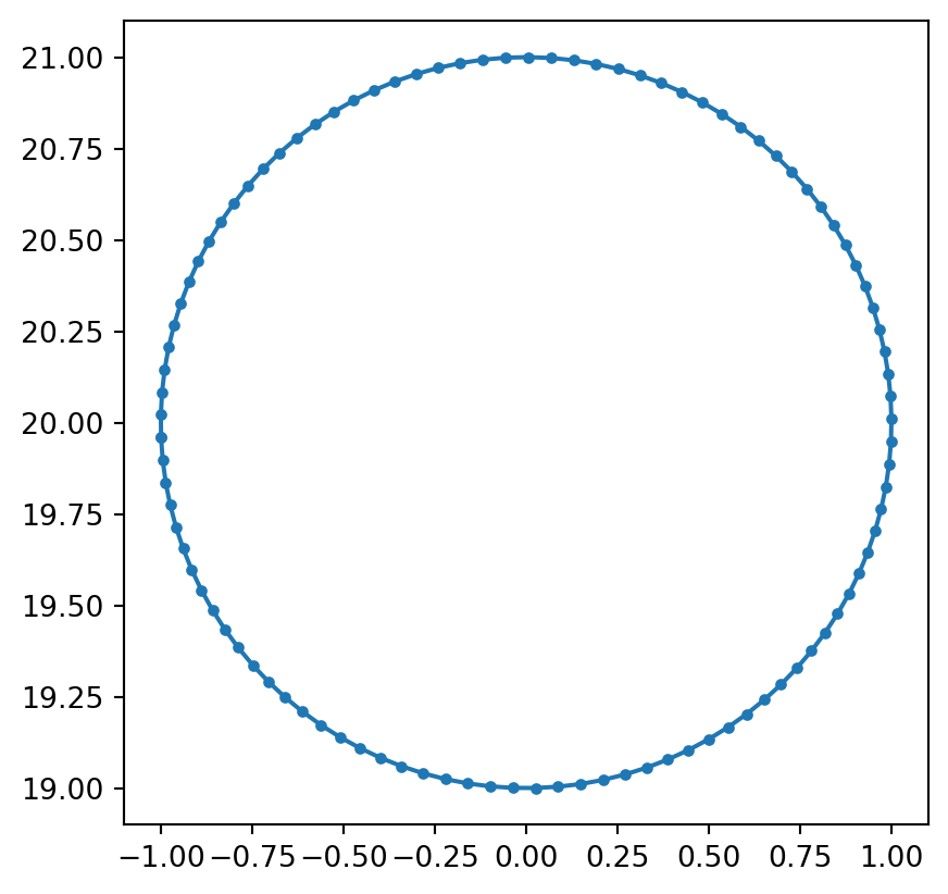
Show the code
def talwani(obs, polygon):
    gz = 0.0
    density = polygon.density
    x = polygon.x
    z = polygon.z
    n = polygon.n
    xp = obs[0]
    zp = obs[1]
    for k in range(n):   
        xv = x[k] - xp
        zv = z[k] - zp
        xvp1 = x[k+1] - xp
        zvp1 = z[k+1] - zp
        if not isclose(zv, zvp1):
            a_i = xvp1 + zvp1 * (xvp1 - xv) / (zv - zvp1)
        theta_v = np.arctan2(zv, xv)
        theta_vp1 = np.arctan2(zvp1, xvp1)
        phi_i = np.arctan2(zvp1 - zv, xvp1 - xv)
        
        if theta_v < 0:
            theta_v += np.pi
        if theta_vp1 < 0:
            theta_vp1 += np.pi
            
        if isclose(xv, 0.0): # A
            Zi = -a_i * np.sin(phi_i) * np.cos(phi_i) * (
                theta_vp1 - np.pi/2 + np.tan(phi_i) * np.log(np.cos(theta_vp1) * (np.tan(theta_vp1) - np.tan(phi_i))))
        elif isclose(xvp1, 0.0): # B
            Zi = a_i * np.sin(phi_i) * np.cos(phi_i) * (
                theta_v - np.pi/2 + np.tan(phi_i) * np.log(np.cos(theta_v) * (np.tan(theta_v) - np.tan(phi_i))))
        elif isclose(zv, zvp1): # C
            Zi = zv * (theta_vp1 - theta_v)
        elif isclose(xv, xvp1): # D
            Zi = xv * np.log(np.cos(theta_v) / np.cos(theta_vp1))
        elif isclose(theta_v, theta_vp1): # E
            Zi = 0.0
        elif isclose(xv, zv): # F
            Zi = 0.0
        elif isclose(xvp1, zvp1): # G
            Zi = 0.0
        else:
            a_i = xvp1 + zvp1 * (xvp1 - xv) / (zv - zvp1)
            Zi = a_i * np.sin(phi_i) * np.cos(phi_i) * ( 
            theta_v - theta_vp1 + np.tan(phi_i) * 
            np.log( 
                np.cos(theta_v) * ( np.tan(theta_v) - np.tan(phi_i) ) /
                np.cos(theta_vp1) / ( np.tan(theta_vp1) - np.tan(phi_i) )))
        gz += Zi
    gz = gz * 2 * 6.674e-11 * density
    return gz

\[ Z_{i} =a_{1} \sin \phi_{i} \cos \phi_{i} \left[ \theta_{i}-\theta_{i+1} +\tan \phi_{i} \log _{s} \frac{\cos \theta_{i}\left(\tan \theta_{i}-\tan \phi_{j}\right)}{\cos \theta_{i+1}\left(\tan \theta_{i+1}-\tan \phi_{i}\right)}\right] \]

11.1 Numerical experiment

We define a cylinder of radius \(r=1\) that will be approximated in the \(x-z\)-plane by a sufficiently large number of line segments around its enclosing circle.

Show the code
n = 101
xc = 0.0
zc = 20.0
radius = 1.0
x = np.array([xc + radius * np.cos(0.01 + 2 * np.pi * k / n) for k in np.linspace(0, n-1, n)])
z = np.array([zc + radius * np.sin(0.01 + 2 * np.pi * k / n) for k in np.linspace(0, n-1, n)])
poly = Polygon(x, z, 500)
Show the code
fig, ax = plt.subplots()
plt.plot(poly.x, poly.z, marker='.')
ax.set_aspect('equal', 'box');

We define a profile perpendicular to the strike of the cylinder.

The arrays gtal and gcyl store the values obtained by the Talwani method and the analytical solution for the cylinder, respectively.

Show the code
profile = np.linspace(start=-40, stop=40, num=81)
npts = profile.size
gtal = np.zeros(npts)
gcyl = np.zeros(npts)
mass = poly.density * np.pi * radius**2
for k in range(npts):
    gtal[k] = talwani(np.array([profile[k], 0]), poly)
    gcyl[k] = cylinder(np.array([profile[k], 0]), mass, np.array([xc, zc]))[1]

The following plots illustrate the accuracy of the Talwani approach.

Show the code
fig, (ax1, ax2) = plt.subplots(1, 2)
ax1.plot(profile, gtal, marker='.')
ax1.plot(profile, gcyl, marker='.')
ax2.plot(profile, gcyl - gtal, marker='.')
ax1.set_title('anomaly')
ax2.set_title('difference');

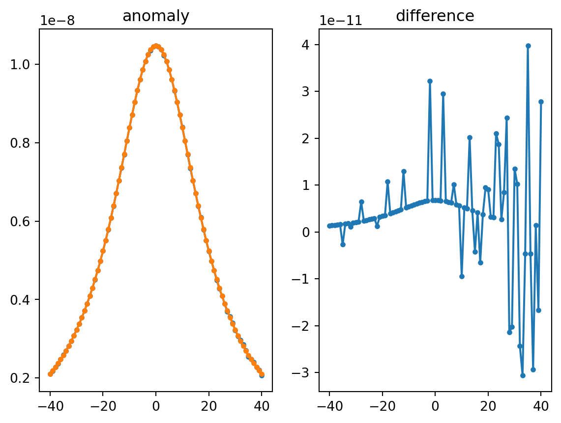
Comparison of analytical and numerical solutions (left) and absolute difference (right).

The relative error is

Show the code
print(norm(gtal - gcyl) / norm(gcyl))
0.0018837709519435105