21  Numerical computation of Legendre polynomials

Show the code
import numpy as np
from sympy import symbols, factorial, Derivative, series, lambdify, simplify, factor, expand, collect
from sympy import sin, cos, sqrt, latex, binomial, Rational, summation
import matplotlib.pyplot as plt
import cartopy
import cartopy.crs as ccrs
from IPython.display import display, Math

mydisplay = lambda pre, ex, post: display(Math(pre + latex(ex) + post))

The Legendre polynomials were first introduced in 1782 by Adrian-Marie Legendre as the coefficients in the expansion of the Newtonian potential.

In this section we demonstrate how the Legendre polynomials can be computed.

A very handy and especially compact expression for the Legendre polynomials is given by the formula of Rodrigues

\[ P_n(x) = \frac{1}{2^n n!} \frac{\mathrm d^n}{\mathrm dx^n} (x^2 - 1)^n. \]

It is straightforward to compute these polynomials with the help of SymPy.

We implement the above equation and later substitute \(x=:\cos\theta\).

First, we introduce symbolic variables.

Show the code
x, theta = symbols('x theta', real=True)
n = symbols('n', integer=True, nonnegative=True)

Next, we define a symbolic expression which provides (not evaluates) the formula of Rodrigues. Note that we introduce a symbolic differentiation (up to order n) by using the Derivative function. The differentiation can later be carried out explicitly by calling the method .doit().

Show the code
Pn = 1 / ( 2**n * factorial(n)) * Derivative((x**2 - 1)**n, (x, n))
mydisplay('P_n(x) = ', Pn, '')

\(\displaystyle P_n(x) = \frac{2^{- n} \frac{d^{n}}{d x^{n}} \left(x^{2} - 1\right)^{n}}{n!}\)

Let’s evaluate the Legendre polynomials \(P_n(\cos\theta)\) for a small range of order \(n\), say \(0 \le n \le 5\).

Note: - First, we iterate through a list of orders n (for i in range(0,5):) and substitute the desired value of n with i (subs(n, i)) - Second, with the fixed order of the derivative, we carry out the differentiation by calling doit() - Finally, we substitute x with cos(theta) and expand the expression.

Show the code
for i in range(0,5):
    mydisplay('P_' + str(i) + '(\\cos\\theta) = ', Pn.subs(n, i).doit().subs(x, cos(theta)).expand(), '')

\(\displaystyle P_0(\cos\theta) = 1\)

\(\displaystyle P_1(\cos\theta) = \cos{\left(\theta \right)}\)

\(\displaystyle P_2(\cos\theta) = \frac{3 \cos^{2}{\left(\theta \right)}}{2} - \frac{1}{2}\)

\(\displaystyle P_3(\cos\theta) = \frac{5 \cos^{3}{\left(\theta \right)}}{2} - \frac{3 \cos{\left(\theta \right)}}{2}\)

\(\displaystyle P_4(\cos\theta) = \frac{35 \cos^{4}{\left(\theta \right)}}{8} - \frac{15 \cos^{2}{\left(\theta \right)}}{4} + \frac{3}{8}\)

We observe that Legendre polynomials are polynomials in \(\cos\theta\).
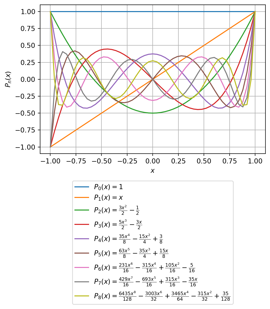
Let’s visualize:

Show the code
xx = np.linspace(-1, 1, 51)
ax, fig = plt.subplots(figsize=(6,4))
for i in range(0, 9):
    ex = Pn.subs(n, i).doit().expand()
    f = lambdify(x, ex, "numpy")
    yy = np.array([f(p) for p in xx])
    plt.plot(xx, yy, label=f"$P_{i}(x) = $" + f"${latex(ex)}$")
    plt.xlabel(r'$x$')
    plt.ylabel(r'$P_n(x)$')
    plt.grid(True)
plt.legend(loc='upper center', bbox_to_anchor=(0.5, -0.16));

Legendre polynomials up to degree 8

In the following we reproduce these results by expanding the inverse distance \(1/r\), which is the main feature of, e.g., the potential of a point mass in \(\mathbb R^3\).

The gravity potential due to a point mass \(m\) located at the point \(\mathbf r'\) observed at the point \(\mathbf r\) is given by

\[ V(\mathbf r) = -f \frac{m}{|\mathbf r - \mathbf r'|} \]

Note that the point mass is not in the center of a sphere, but has been moved slightly along the \(z\)-axis to the point \(\mathbf r' = (0, 0, s)^\top\).

The term \(1/|\mathbf r - \mathbf r'|\) can be expanded in a Taylor series when \(|\mathbf r'| \ll |\mathbf r|\).

Let \(\mathbf r = (x, y, z)^\top\) and \(\mathbf r' = (0, 0, s)^\top\). The Euclidean distance between the point mass and the point of observation is \(q = |\mathbf r - \mathbf r'|\). With \(r = |\mathbf r|\) and \(s = |\mathbf r'|\) we can rewrite the term \(1/q\) using the Theorem of Cosines as

\[ \frac{1}{q}=f(r, \theta)=\frac{1}{r}\left[1+\left(\frac{s}{r}\right)^{2}-2 \frac{s}{r} \cos \theta\right]^{-1 / 2} \]

When \(s \ll r\), we can expand \(f(r, \theta)\) in a binomial series as

\[ f(r, \theta) = \frac{1}{r} (1 + b)^{-1/2} = \frac{1}{r}\sum\limits_{n=0}^\infty \left( -1/2 \atop n \right)b^n \] with \[ b = \left(\frac{s}{r}\right)^2 - 2 \frac{s}{r}\cos\theta, \quad |b| < 1 \]

Rearranging after powers of \(s/r\) we arrive at

\[ f(r, \theta) = \frac{1}{r} \sum\limits_{n=0}^\infty\left(\frac{s}{r} \right)^n P_n(\cos\theta) \]

The \(P_n(\cos\theta)\) are polynomials of degree \(n\) in \(\cos\theta\).

The polynomial coefficients in the binomial series are binomial coefficients given by \[ \left( -1/2 \atop n \right) \] The binomial coefficients for \(0 \le n \le 4\) are:

Show the code
[binomial(Rational(-1, 2), i) for i in range(0, 5)]
[1, -1/2, 3/8, -5/16, 35/128]

Next, we expand \[ f(r, \theta) = \frac{1}{r \sqrt{1 + \left(\dfrac{s}{r}\right)^2 - 2 \dfrac{s}{r}\cos\theta}} \] into a series. To this end, we define a symbolic expression for \(f\).

Show the code
r, s, b = symbols('r s b')
f = 1 / r / sqrt(1 + b)
mydisplay('f(b) = ', f, '')

\(\displaystyle f(b) = \frac{1}{r \sqrt{b + 1}}\)

We expand in a power series of \(b\):

Show the code
series(f, b, n=3).removeO().collect(s/r).expand(basic=True)

\(\displaystyle \frac{3 b^{2}}{8 r} - \frac{b}{2 r} + \frac{1}{r}\)

We repeat this step, but replace b to obtain the following result:

Show the code
series(f, b, n=4).removeO().subs(b, (s/r)**2 -2*s/r*cos(theta)).collect(cos(theta)).collect(s/r).expand()

\(\displaystyle \frac{1}{r} + \frac{s \cos{\left(\theta \right)}}{r^{2}} + \frac{3 s^{2} \cos^{2}{\left(\theta \right)}}{2 r^{3}} - \frac{s^{2}}{2 r^{3}} + \frac{5 s^{3} \cos^{3}{\left(\theta \right)}}{2 r^{4}} - \frac{3 s^{3} \cos{\left(\theta \right)}}{2 r^{4}} - \frac{15 s^{4} \cos^{2}{\left(\theta \right)}}{4 r^{5}} + \frac{3 s^{4}}{8 r^{5}} + \frac{15 s^{5} \cos{\left(\theta \right)}}{8 r^{6}} - \frac{5 s^{6}}{16 r^{7}}\)

This is a polynomial in \(\cos\theta\). The coefficients have the form \(\dfrac{1}{r}\left(\dfrac{s}{r}\right)^n\).

The following cell forms the expression \[ \sum_{n=0}^\infty \left( -1/2 \atop n \right) b^n \] (Note that we have omitted the leading term \(1/r\)).

Show the code
b = (s / r)**2 - 2 * s / r * cos(theta)
expand(summation(binomial(Rational(-1, 2), n) * b**n, (n, 0, 3))).collect(s/r).expand()

\(\displaystyle 1 + \frac{s \cos{\left(\theta \right)}}{r} + \frac{3 s^{2} \cos^{2}{\left(\theta \right)}}{2 r^{2}} - \frac{s^{2}}{2 r^{2}} + \frac{5 s^{3} \cos^{3}{\left(\theta \right)}}{2 r^{3}} - \frac{3 s^{3} \cos{\left(\theta \right)}}{2 r^{3}} - \frac{15 s^{4} \cos^{2}{\left(\theta \right)}}{4 r^{4}} + \frac{3 s^{4}}{8 r^{4}} + \frac{15 s^{5} \cos{\left(\theta \right)}}{8 r^{5}} - \frac{5 s^{6}}{16 r^{6}}\)

This is — up to the leading term — the same expression that we have derived above by a series expansion of \(f(r, \theta)\).

It can be demonstrated that similar results can be obtained when we form the summation \[ \sum_{n=0}^\infty \left( \frac{s}{r}\right)^n \, P_n(\cos\theta) \]

(Note that the number of terms differs when we stop the summation for a finite value of \(n\).)

Show the code
ss = 1
for i in range(1,6):
    ss = ss + (s/r)**i * Pn.subs(n, i).doit().subs(x, cos(theta))
display(simplify(ss).collect(cos(theta)).expand().subs(sin(theta)**2, 1 - cos(theta)**2).collect(s/r).expand())

\(\displaystyle 1 + \frac{s \cos{\left(\theta \right)}}{r} + \frac{3 s^{2} \cos^{2}{\left(\theta \right)}}{2 r^{2}} - \frac{s^{2}}{2 r^{2}} + \frac{5 s^{3} \cos^{3}{\left(\theta \right)}}{2 r^{3}} - \frac{3 s^{3} \cos{\left(\theta \right)}}{2 r^{3}} + \frac{35 s^{4} \cos^{4}{\left(\theta \right)}}{8 r^{4}} - \frac{15 s^{4} \cos^{2}{\left(\theta \right)}}{4 r^{4}} + \frac{3 s^{4}}{8 r^{4}} + \frac{63 s^{5} \cos^{5}{\left(\theta \right)}}{8 r^{5}} - \frac{35 s^{5} \cos^{3}{\left(\theta \right)}}{4 r^{5}} + \frac{15 s^{5} \cos{\left(\theta \right)}}{8 r^{5}}\)

21.1 Visualization on a sphere

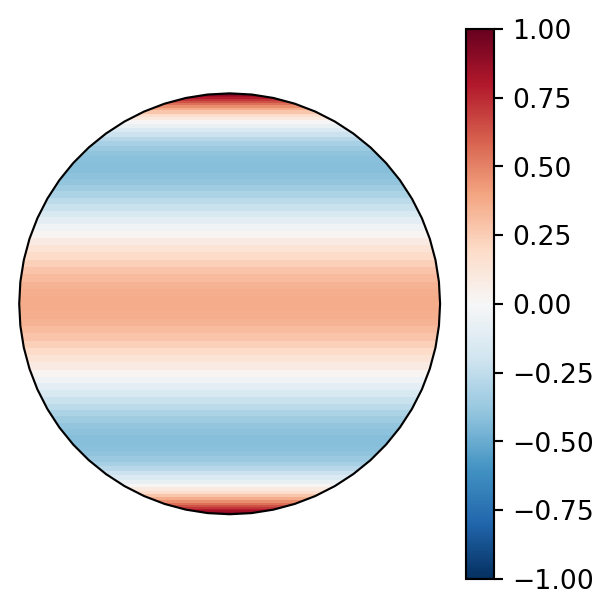
We illustrate the Legendre polynomials on the surface of a sphere, i.e., for \(r=const\). The potential function is a function of \(\theta\) only. Hence, Legendre polynomials are referred to as zonal spherical harmonics.

Let’s plot \(P_4(\cos\theta)\):

Show the code
deg2rad = lambda x: x * np.pi / 180.0

m = 4
ex = Pn.subs(n, m).doit().subs(x, cos(theta))
legendreP = lambdify(theta, ex, "numpy")

lon = np.linspace(0, 360.0, 180) - 180.0
lat = np.linspace(-90.0, 90.0, 90)
colat = lat + 90.0
d = np.zeros((len(lon), len(colat)), dtype = np.float64)
for j, yy in enumerate(colat):
    for i in range(len(lon)):
        d[i, j] = legendreP(deg2rad(yy))
drm = np.transpose(d)
Show the code
fig = plt.figure(figsize=(3, 3),tight_layout = {'pad': 0})
plotcrs = ccrs.Orthographic(0, 0)
ax = plt.subplot(projection=plotcrs)
cf = ax.pcolormesh(lon, lat, drm,
    transform=ccrs.PlateCarree(),
    cmap='RdBu_r', vmin=-1, vmax=1)
plt.colorbar(cf)
ax.relim()
ax.autoscale_view()

21.2 Summary

The Legendre polynomials can be defined as the coefficients in a formal expansion in powers of \(t\) of the generating function \[ \frac{1}{\sqrt{1-2xt+t^2}} = \sum_{n=0}^\infty P_n(x) t^n. \] The coefficient of \(t^n\) is a polynomial in \(x\) of degree \(n\) with \(|x| \le 1\).

In our approach outlined above, we have set \[ t =: \frac{s}{r} \] and \[ x =: \cos\theta. \]

A further definiton of the Legendre polynomials is given in terms of solutions to Legendre’s differential equation \[ (1 - t^2) P_n''(x) - 2 x P_n'(x) + n(n+1) P_n(x) = 0. \]