8  Circular Disc

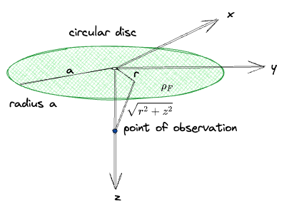
We consider the potential and gravitational attraction of a circular disc in the plane \(z=0\) aligned with the z axis.

Figure 8.1: A circular disc of radius \(a\) aligned with the axis \(z=0\).

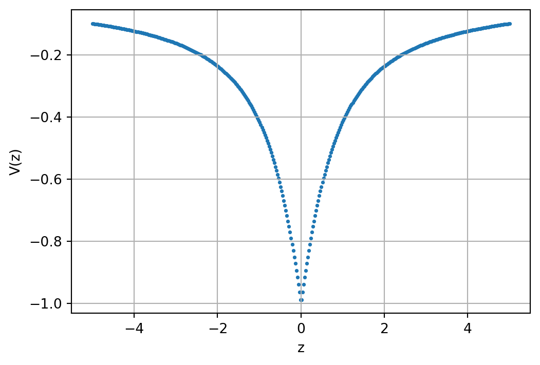
8.1 Potential along the z axis

To obtain the potential at the \(z\)-axis we integrate over the surface area of the disc: \[ V(z) = -f \frac{m}{r} = -2 \pi f \rho_F \int\limits_{r=0}^a \frac{r \, \dd r}{\sqrt{ r^2 + z^2 }} \] with \(r^2 = x^2 + y^2\).

Integration yields: \[ V(z) = 2 \pi f (|z| - \sqrt{ a^2 + z^2 }) \]

Sympy check:

Show the code
import sympy as sp
from sympy import pi, oo
x, y, z = sp.symbols('x y z', real=True)
r, f, a, rho = sp.symbols('r f a rho_F', real=True, positive=True)

V = sp.integrate(-2 * pi * f *rho * r / sp.sqrt(r**2 + z**2), (r, 0, a))
V.simplify()

\(\displaystyle 2 \pi f \rho_{F} \left(- \sqrt{a^{2} + z^{2}} + \left|{z}\right|\right)\)

Show the code
import numpy as np
import matplotlib.pyplot as plt

zz = np.linspace(-5, 5, 400)
fig, ax = plt.subplots(figsize=(6,4))
plt.scatter(zz, np.abs(zz) - np.sqrt(1 + zz**2),s=3)
plt.grid(True)
plt.xlabel('z')
plt.ylabel('V(z)');
Figure 8.2: Potential of a circular disc of radius \(a\) at \(z=0\).

8.2 Gravitational attraction along the z axis

The vertical component of the gravitational attraction is the projection of the field \(\vb g\) onto the vertical direction \(\hat{\vb e}_z\)

\[ \vb g(z) = -\grad V(z) \]

\[ -\grad V(z) \cdot \hat{\vb e}_z = -\pdv{}{z}V(z) = 2 \pi f \rho_F \left( \frac{z}{\sqrt{ a^2 + z^2 }} - \text{sign}(z) \right) \]

This is the attraction of a disc of density \(\rho_{F}\) aligned with the plane \(z=0\) observed at some point at the \(z\) axis.

Sympy check:

Show the code
g = -sp.diff(V, z)
g

\(\displaystyle \frac{2 \pi f \rho_{F} z}{\sqrt{a^{2} + z^{2}}} - 2 \pi f \rho_{F} \operatorname{sign}{\left(z \right)}\)

Note

Note that

\[ \dv{|z|}{z} = \text{sign}z. \]

Show the code
fig, ax = plt.subplots(figsize=(6,4))
plt.scatter(zz, 2 * np.pi * (zz / np.sqrt(1 + zz**2) - np.sign(zz)),s=3)
plt.xlabel('z')
plt.ylabel('g(z)')
plt.grid(True);
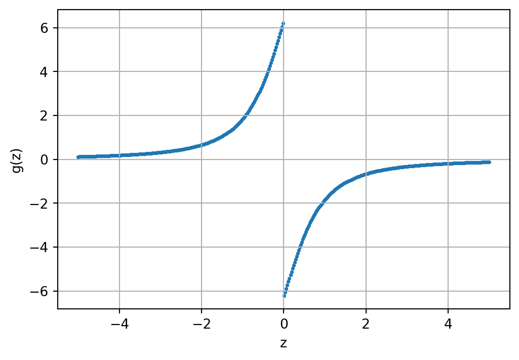
Figure 8.3: Vertical attraction of a circular disc of radius \(a\) coplanar with \(z=0\).

The vertical component of the gravitational attraction obviously has a jump, which equals \(4 \pi f \rho_F\).

Show the code
sp.limit(g, z, 0, '-') - sp.limit(g, z, 0, '+')

\(\displaystyle 4 \pi f \rho_{F}\)

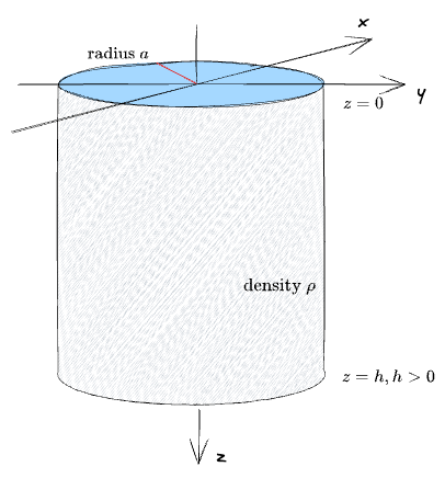
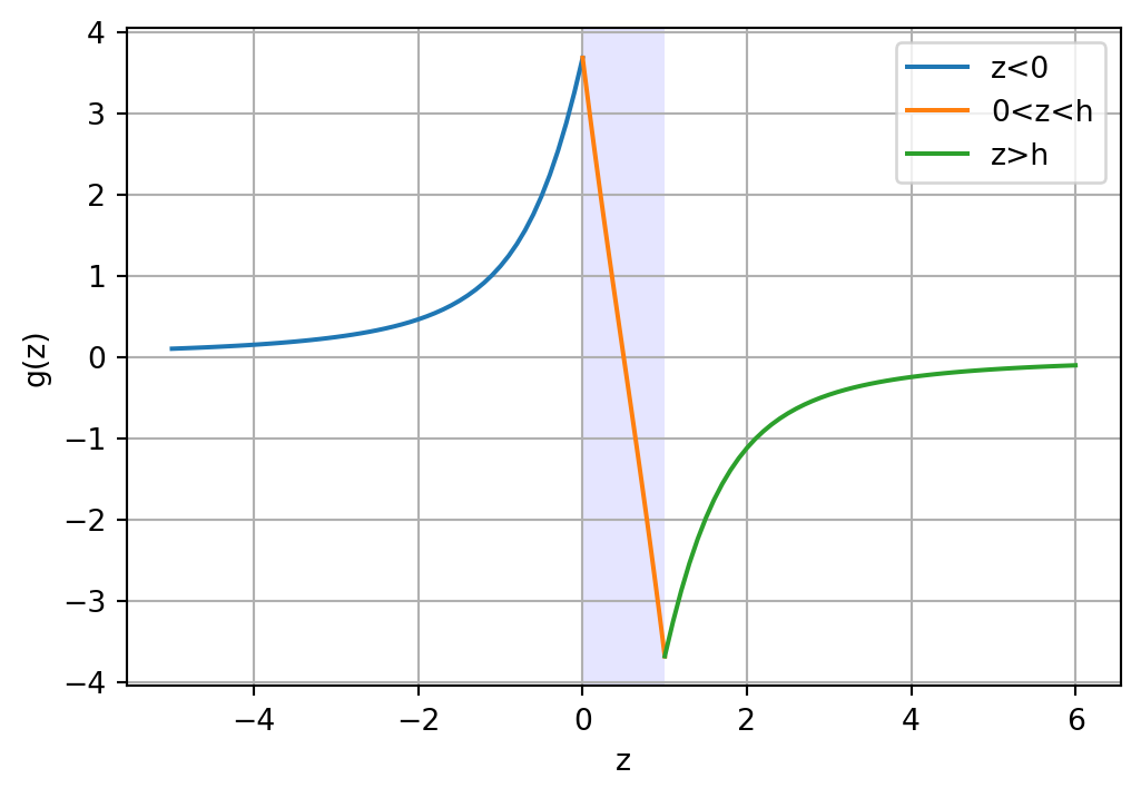
8.3 Potential and attraction of a vertical cylinder

The cylinder is composed of circular discs with infinitely small thickness and constant radius \(a\). The integration of an aligned stack of such discs yields a cylinder.

Figure 8.4: A co-axial stack of circular discs from \(z=\) to \(z=h\) forming a vertical cylinder of length \(h\).

We note that

\[ \rho = \int_0^h \rho_F \, \dd z. \]

We integrate over the attraction for circular discs and obtain for a cylinder enclosed by the two horizontal planes \(z=0\) and \(z=h, h>0\): \[ \begin{align} g(z) & = 2 \pi f \rho \left(h + \sqrt{ a^2 + z^2 } - \sqrt{ a^2 + (h - z)^{2} }\right) \qfor z < 0 \\ & = 2 \pi f \rho \left(h - 2z + \sqrt{ a^{2} + z^{2}} - \sqrt{ a^2 + (h-z)^{2} }\right) \qfor h > z \\ & = 2 \pi f \rho \left(-h + \sqrt{ a^2 + z^2 } - \sqrt{ a^2 + (h - z)^{2} }\right) \quad\text{otherwise} \end{align} \]

Sympy check:

Show the code
h = sp.symbols('h', real=True, positive=True)
rho0 = sp.symbols('rho', real=True, positive=True)
i1 = sp.integrate(-g, z).subs(rho, rho0)
sp.simplify(i1.subs(z, z-h) - i1.subs(z, z-0))

\(\displaystyle \begin{cases} 2 \pi f \rho \left(h + \sqrt{a^{2} + z^{2}} - \sqrt{a^{2} + \left(h - z\right)^{2}}\right) & \text{for}\: z < 0 \\2 \pi f \rho \left(h - 2 z + \sqrt{a^{2} + z^{2}} - \sqrt{a^{2} + \left(h - z\right)^{2}}\right) & \text{for}\: h > z \\2 \pi f \rho \left(- h + \sqrt{a^{2} + z^{2}} - \sqrt{a^{2} + \left(h - z\right)^{2}}\right) & \text{otherwise} \end{cases}\)

Show the code
hh = 1.0
zabove = np.linspace(-5, 0, 51)
zinside = np.linspace(0, hh, 51)
zbelow = np.linspace(hh, 6, 51)
fig, ax = plt.subplots(figsize=(6,4))
plt.plot(zabove, 
         2*np.pi*(hh + np.sqrt(1+zabove**2) - 
                  np.sqrt(1 + (hh - zabove)**2)),c='C0',
        label=r'z<0')
plt.plot(zinside, 
        2*np.pi*(hh - 2 * zinside + np.sqrt(1+zinside**2) - 
                 np.sqrt(1 + (hh - zinside)**2)),c='C1',
        label=r'0<z<h')
plt.plot(zbelow, 
         2*np.pi*(-hh + np.sqrt(1+zbelow**2) - 
                  np.sqrt(1 + (hh - zbelow)**2)),c='C2',
        label=r'z>h')
plt.axvspan(0, hh, facecolor='b', alpha=0.1)
plt.xlabel('z')
plt.ylabel('g(z)')
plt.legend()
plt.grid(True);

8.4 Bouguer plate anomaly

Consider the solution for \(z<0\). What happens to \(g(z)\) when \(a\) goes to infinity, i.e., the cylinder turns into an infinite horizontal plate? We depart from the first of the above equations. In \(z<0\) we have \[ g(z) = 2 \pi f \rho \left( h + \sqrt{ a^2 + z^2 } - \sqrt{ a^2 + (h - z)^2 }\right) \] For \(a \to \infty\) we can expand the square root into a series, e.g. \[ \sqrt{ a^2 + z^2 } = a \sqrt{ 1 + \frac{z^2}{a^2} } \approx a \left( 1 + \frac{z^2}{2a^2} - \dots\right) \] and \[ \sqrt{ a^2 + (h-z)^2 } = a \sqrt{ 1 + \frac{(h-z)^2}{a^2} } \approx a \left( 1 + \frac{(h-z)^2}{2a^2} - \dots\right) \] After collecting terms we have \[ g(z) = 2 \pi f \rho \left(h + a \left[ 1 + \frac{z^2}{2a^2} - 1 - \frac{(h-z)^2}{a^2}\right]\right) \approx 2 \pi f \rho_{F}h \] This is the well-known equation for the vertical attraction above an infinite horozontal plate of thickness \(h\) and density \(\rho\) (Bouguer plate anomaly)

\[ g_B(h) = 2 \pi f \rho h \]