A vector field \(\vb F : \mathbb R^n \mapsto \mathbb R^n\) defined on a subset \(\Omega \subset \mathbb R^n\) assigns to each point \(\vb x \in \mathbb R^n\) a vector \(\vb F(\vb x) \in \Omega\).
A vector field \(\vb F\) is a potential or conservative vector field if and only if there exists a scalar field \(\Phi: \mathbb R^n \mapsto \mathbb R\) such that it holds \(\vb F (\vb x) = \grad \Phi(\vb x)\).
2.1.2 Equivalent properties of conservative fields
The line integral \(\int_C\) along any curve \(C\) within the field only depends on the start and the end points, but not on the path between them (path independence)
The closed line integral is zero for any curve \(C\): \(\oint_C \grad \Phi(\vb x ) \cdot \dd{\vb x} = \oint \vb F (\vb x ) \cdot \dd{\vb x} = 0\)
Such vector fields are curl free (irrotational), i.e., \(\curl \grad \Phi(\vb x ) = \curl \vb F (\vb x ) \equiv \vb 0\)
2.1.3 Divergence theorem
Statements about the sources and sinks of vector fields can be derived by applying the divergence theorem.
The dielectric displacement \(\vb D = \varepsilon(\vb x) \vb E(\vb x)\) has its sources in a volume density of electric charges \(\rho_E (\vb x)\).
For homogeneous dielectrics we obtain the Poisson equation of electrostatics
\(-\Delta \Phi = \rho_E/\varepsilon.\)
2.1.4 Poisson equation
Potential theory attempts to calculate the unknown potential (the potential function) \(\Phi\) caused by a given physical quantity, e.g., a source distribution \(\rho(\vb x)\).
The potential function can generally be determined by integrating the Poisson equation.
Often, only its spatial derivative is desired, because for physicists only the fields are a meaningful quantity.
2.1.5 Laplace equation
In a region where sources are absent, i.e., \(\rho(\vb x ) \equiv 0\), the Poisson equation becomes the Laplace equation
\(\Delta \Phi(\vb x) = 0\)
with the scalar function \(\Phi\) (the potential) defined over a subset \(\Omega \subset \mathbb R^n\).
This elliptic partial differential equation (or short, the potential equation) is the point of departure in the potential theory.
2.1.6 Mathematical Tools
The potential theory makes use of the functional analysis and its tools, e.g.,
vector spaces
inner product
norm
differentiability
continuity
etc.
TipSpaces
We consider spaces with a norm induced by the inner product.
Euclidean space: Any vector space defined over \(\mathbb R^n\) equipped with an inner product of any finite dimension is called Euclidean vector space.
The coordinate space \(\mathbb R^3\) with standard dot product is a Euclidean space!
Hilbert space: A Hilbert space is a vector space \(H\) with an inner product \(\langle f,g \rangle\) such that the norm \(|f| = \langle f,f \rangle^{1/2}\) turns the space into a complete metric space.
The coordinate spaces \(\mathbb R^n\) and \(\mathbb C^n\) are Hilbert spaces!
TipScalar product
With \(\vb x = (x_1, x_2, \dots, x_n)^\top\) we denote an \(n\)-tuple of numbers or a point in \(\mathbb R^n\), and define the scalar product in \(\mathbb R^n\) given by the dot product
\[
\langle \cdot,\cdot \rangle : \mathbb R^n \mapsto \mathbb R,
\] e.g., \[
\langle \vb x , \vb y \rangle = \sum_{i=1}^n x_i y_i
\] as well as the norm induced by the inner product\[
x = \abs{\vb x} = \langle \vb x , \vb x \rangle^{1/2}
\] The norm \(\abs{\cdot} : \mathbb R^n \mapsto \mathbb R\), as a function, assigns to \(\vb x\) its length.
TipDifferentiation
Let \(\Omega \subset \mathbb R^n\) be an open subset.
A derivative of order\(\vb \alpha\) is defined by a differential operator \(D: C^k (\Omega) \mapsto C(\Omega)\) represented by
and a multi-index\(\vb(\alpha = (\alpha_1, \alpha_2, \dots, \alpha_n) \in \mathbb N_0^n\) with \(|\vb\alpha| = \sum_{i=1}^n \alpha_i\).
Other notations derived from the above definition are:
\(f_x := \pdv{f}{x}\) where \(n=1, \alpha_1=1, |\vb\alpha|=1\)
\(f_{x x} := \pdv[2]{f}{x}\) where \(n=1, \alpha_1=2, |\vb\alpha|=2\)
\(f_{x z} := \pdv{f}{x}{z}\) where \(n=3, \alpha_1=1, \alpha_2=0, \alpha_3=1, |\vb\alpha||=2\)
TipDifferentiability classes
What is \(C^k(\Omega)\)?
The space of the continuous real valued functions in a domain \(\Omega\) is of class \(C(\Omega)\) or \(C^0(\Omega)\).
This space contains all differentiable functions in \(\Omega \subset \mathbb R^n\).
Functions whose (partial) derivatives are also continuous are called continuously differentiable. These functions are said to be of class \(C^1(\Omega)\).
Correspondingly, \(C^n (\Omega)\) is called the space of the functions which are \(n\)-differentiable, where the \(n\)-th derivative \(D^{\vb\alpha} f(\vb x), |\vb\alpha| \le n\) is continuous on \(\Omega\).
Arbitrarily often differentiable (smooth) functions belong to \(C^\infty ( \Omega)\).
TipHarmonic function
We define the harmonic function:
A real-valued function \(U(\vb x) \in C^2 (\Omega)\) is called harmonic or regular potential function in the subset \(\Omega \subset \mathbb R^n\) if there holds
\[
\Delta U(\vb x) = 0
\]
for \(\vb x \in \Omega\).
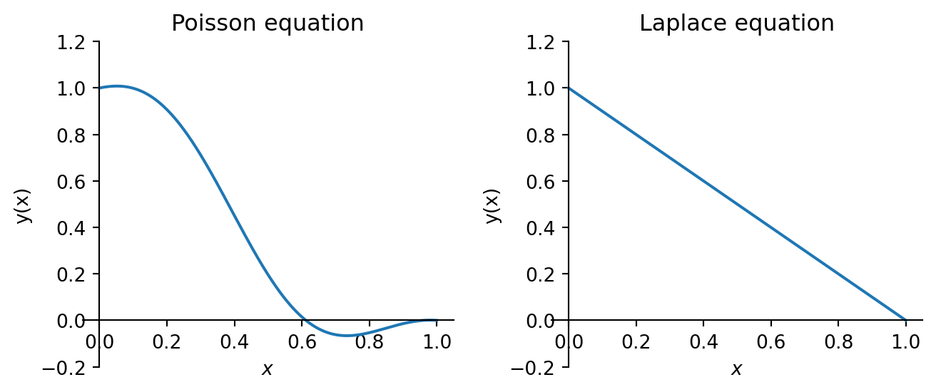
2.2 Solution of the Laplace and Poisson equations
We consider the second-order differential equations
TipLaplace equation
\[
\dv[2]{y}{x} = 0
\]
and
TipPoisson equation
\[
\dv[2]{y}{x} = -4\cos(4x) - 8 \sin(8 x)
\]
for \(x \in [0, 1]\) subject to the boundary conditions \(y(0)=1\) and \(y(1)=0\).
To obtain the solution to the above PDEs, we employ the Python package sympy, which is a powerful library for symbolic mathematics.
Symbolic functions which depend on symbolic variables have to be defined with the function Function.
The solution of the differential equations can be obtained by a call to the dsolve function.
The signature of the function can be understood as follows:
Solve the symbolic equation given by the expressions eq_poisson and eq_laplace, resp.
The desired solution is y(x)
Boundary conditions can be enforced by the values following the keyword ics. In the example, y(0)=1 and y(1)=0.
The solution of the Laplace equation does not exhibit local extrema
It has no curvature
The solution of the Poisson equation has local minima and maxima
Its extrema might get larger or smaller than those of the Dirichlet values at the boundary
2.4 Mean value theorem
We observe an important property of harmonic functions:
A continuous function \(f: \Omega \subset \mathbb R_{n} \mapsto \mathbb R\) is a harmonic function, if there holds
\[
f(\mathbf{x}) = \frac{1}{r^{n-1}s_{n}} \int_{\partial K(\mathbf{x}, r)} f(\mathbf{y}) \, \mathrm d \sigma(\mathbf{y})
\] for any sphere \(K(\mathbf{x}, r)\) of radius \(r\) in \(\mathbf{x}\) enclosed by \(\Omega\). \(s_{n}\) is the surface measure of the n-dimansional unit sphere.
In \(\mathbb R^3\) we have \[
f(\mathbf{x}) = \frac{1}{4 \pi r^{2}} \int_{\partial K(\mathbf{x}, r)} f(\mathbf{y}) \, \mathrm d \sigma(\mathbf{y})
\]
The value of a harmonic function at any given point \(\mathbf{x}\) is the average of its neighboring values.
From the definition of the second derivative we can infer an alternative approach for the 1-D case:
From the definition of the second derivative \[
\frac{\mathrm d^{2}\Phi(x)}{\mathrm d x^{2}} = \lim_{\Delta x \to 0}
\frac{\Phi(x + \Delta x) - 2 \Phi(x) + \Phi(x - \Delta x)}{\Delta x^{2}}
\] we obtain \[
\lim_{\Delta x \to 0} \frac{1}{\Delta x^{2}} \left(
\Phi(x) - \frac{1}{2}(\Phi(x - \Delta x) + \Phi(x + \Delta x))
\right) = -\frac{1}{2}\frac{\mathrm d^{2}\Phi}{\mathrm d x^{2}}
\] from which it follows that \[
\Phi(x) = \frac{1}{2} \lim_{\Delta x \to 0}
(\Phi(x - \Delta x) + \Phi(x + \Delta x)).
\]
2.5 Min-Max Property
From the mean value theorem follows the min-max property, which states that the solution \(\Phi\) of the Laplace equation in a closed domain \(\Omega\) never has its minimum and maximum values in its interior.
\[
\begin{align}
\max(\Phi(x), x \in \Omega) & \lt \max(\Phi(x), x \in \overline{\Omega}) = \max(\Phi(x), x \in \partial \Omega) \\
\min(\Phi(x), x \in \partial \Omega) & = \min(\Phi(x), x \in \overline{\Omega}) \lt \min(\Phi(x), x \in \Omega)
\end{align}
\]
Here, \(\overline \Omega\) is the closure of \(\Omega\), which is the smallest closed set containing \(\Omega\).
Equivalently, \[
\overline\Omega = \Omega \cup \partial \Omega
\] where \(\partial\Omega\) denotes the boundary of \(\Omega\).
On the other hand, the domain \(\Omega\) is an open subset of \(\mathbb R^{n}\). Open means that every point \(x \in \Omega\) has a small ball \(B_{\varepsilon}(x)\) that is still contained in \(\Omega\). Thus, the boundary points are not included in \(\Omega\).