6  Plane waves above and inside a homogeneous Earth

In this section we calculate the magnetic and electric fields inside and above a uniform Earth.

We consider plane electromagnetic waves as they are typically used in Magnetotellurics (MT).

The conducting Earth is confined to the halfspace in \(z \ge 0\), whereas the Air halfspace is in \(z < 0\). The electrical conductivity \(\sigma\) of the conducting halfspace is uniform. We use time-harmonic plane waves with a time dependency of \(\exp(i \omega t)\).

The source of electromagnetic induction in the lower halfspace is a homogeneous time-harmonic magnetic field in \(z<0\) with \[ \mathbf H(z, \omega) = \begin{bmatrix} H_x\\ 0\\ 0 \end{bmatrix} e^{i \omega t}, \quad z < 0 \tag{6.1}\]

where the amplitude is \(H_x = 1\) A/m. The inducing field is linear polarized in the \(x\)-direction.

Note

In the following, we drop the term \(e^{i \omega t}\).

What do we know about the magnetic field inside the Earth?

In \(z \ge 0\), the magnetic field is a solution of the Helmholtz equation

\[ \partial^2_{zz} H_x + k^2 H_x = 0, \quad k^2 = - i \omega \mu \sigma \tag{6.2}\]

The solution inside the Earth is

\[ H_x(z) = e^{- i k z} \tag{6.3}\]

Self study

Show that 6.3 is the solution to 6.2!

We now have the complete solution in the entire full-space:

\[ H_x(z) = \begin{cases} 1 & \text{ for } z \le 0 \\ e^{-i k z} & \text{ for } z \ge 0 \end{cases} \]

We have assumed the continuity of \(H_x\) in \(z=0\).

To obtain the electric field associated with the magnetic field in both halfspaces, we make use of Maxwell’s equations.

Recall that in quasi-static approximation,

\[ \curl \mathbf H = \mathbf j. \] More precisely,

\[ \curl \mathbf H = \begin{bmatrix} \partial_x \\ \partial_y \\ \partial_z \end{bmatrix} \times \begin{bmatrix} H_x \\ H_y \\ H_z \end{bmatrix} = \begin{bmatrix} \partial_y H_z - \partial_z H_y \\ \partial_z H_x - \partial_x H_z \\ \partial_x H_y - \partial_y H_x \end{bmatrix}. \]

In our case (cf. 6.1), there is only an \(x\)-component of \(\mathbf H\),

\[ \curl \mathbf H = \begin{bmatrix} 0 \\ \partial_z H_x \\ 0 \end{bmatrix} = \sigma \begin{bmatrix} 0 \\ E_y \\ 0 \end{bmatrix}, \]

which results in a \(y\)-component of the associated electric field \(\mathbf E\). The EM waves \(\mathbf H\) and \(\mathbf E\) are transversal waves, hence mutually orthogonal to the direction of propagation \(\mathbf k\), such that

\[ \mathbf H \perp \mathbf E \perp \mathbf k. \]

Now we derive an expression for \(E_y\) in \(z \ge 0\):

\[ E_y(z) = \frac{1}{\sigma} \partial_z H_x(z) = \frac{ 1 }{ \sigma } \partial_z e^{-i k z} = -\frac{ ik }{ \sigma } e^{-i k z} . \]

The amplitude of the electric field at the surface of the Earth in \(z=0\) is

\[ E_y(0) = -\frac{ ik }{ \sigma }. \]

Tip

\[ \frac{ik}{\sigma} = \frac{ik^2}{k \sigma} = \frac{i(-i\omega\mu_0 \sigma)}{k \sigma} = \frac{\omega\mu_0}{k} \]

Self study

Show that \(E_y(z)\) satisfies Faraday’s law!

Now we turn to the electric field in the Air halfspace, i.e., in \(z\le 0\).

In \(z \le 0\), the magnetic field is uniform with a field intensity of 1 A/m, so

\[ \mathbf H = \begin{bmatrix} 1 \\ 0 \\ 0 \end{bmatrix} \]

We feed this into Faraday’s law:

\[ \curl \mathbf E = \begin{bmatrix} -i \omega \mu \\ 0 \\ 0 \end{bmatrix} = \begin{bmatrix} - \partial_z E_y \\ 0 \\ 0 \end{bmatrix} \]

We see, that to obtain \(E_y\), we have to integrate both sides of

\[ i \omega \mu = \partial_z E_y. \] We integrate by parts and get

\[ \int\limits_0^\xi \partial_z E_y \, \mathrm d z = \left[ E_y \right]_0^\xi = [i \omega \mu]_0^\xi \] Therefore,

\[ E_y(\xi) = E_y(0) + i \omega \mu \xi = -\frac{ \omega\mu_0 }{ k } + i \omega \mu \xi = -\frac{ \omega \mu_0 }{ k } (1 - i k \xi). \]

Finally, we obtain the result

\[ E_y(z) = \begin{cases} -\dfrac{ \omega\mu_0 }{ k } (1 - i k z) & z \le 0 \\ -\dfrac{ \omega\mu_0 }{ k } e^{-i k z} & z \ge 0 \end{cases} \]

Self study

Obtain the appropriate expression for \(E_x(z)\) when \(\vb{H} = [0, 1, 0]^\top\)!

Do you observe a difference? Try to explain your result.

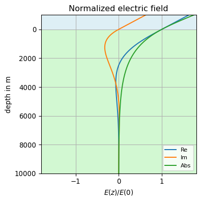
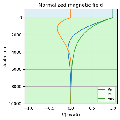
6.1 Visualization

We illustrate our results with a simple example of a uniform halfspace with a conductivity of 0.01 S/m and a frequency of 10 Hz.

Shown are real (Re) and imaginary (Im) part of the fields along with their magnitude (Abs) as a function of depth.

Clearly visible is the exponential decay with depth.

import matplotlib.pyplot as plt
import numpy as np

f = 10
omega = 2 * np.pi * f
sigma = 0.01

z = np.arange(-1000, 10001, 100)

def h(omega, sigma, z):
    k = np.sqrt(-1j * omega * np.pi * 4e-7 * sigma)
    if z < 0:
        H = 1 + 1j * 0
    if z >= 0:
        H = np.exp(-1j * k * z)
    return H

def e(omega, sigma, z):
    k = np.sqrt(-1j * omega * np.pi * 4e-7 * sigma)
    if z < 0:
        E = -1j * k / sigma * (1 - 1j * k * z)
    if z >= 0:
        E = -1j * k / sigma * np.exp(-1j * k * z)
    return E

H = [h(omega, sigma, zz) for zz in z]
E = [e(omega, sigma, zz) for zz in z]
H0 = h(omega, sigma, 0.0)
E0 = e(omega, sigma, 0.0)

In our example, the skin depth is np.float64(1590.63) m.

fig, ax = plt.subplots(figsize=(4, 4), layout='constrained')

ax.plot(np.real(E / E0), z, label='Re')
ax.plot(np.imag(E / E0), z, label='Im')
ax.plot(np.abs(E / E0), z, label='Abs')
ax.axhspan(z[0], 0.0, facecolor='lightblue', alpha=0.4)
ax.axhspan(0.0, z[-1], facecolor='lightgreen', alpha=0.4)
ax.invert_yaxis()
ax.set_ylim((z[-1], z[0]))
ax.set_xlim((-1.8, 1.8))
ax.set_ylabel('depth in m')
ax.set_xlabel(r'$E(z)/E(0)$')
ax.set_title('Normalized electric field')
ax.grid(True)
ax.legend(loc='lower right', fontsize='small', frameon=True)

fig, ax = plt.subplots(figsize=(4, 4), layout='constrained')
ax.plot(np.real(H / H0), z, label='Re')
ax.plot(np.imag(H / H0), z, label='Im')
ax.plot(np.abs(H / H0), z, label='Abs')
ax.axhspan(z[0], 0.0, facecolor='lightblue', alpha=0.4)
ax.axhspan(0.0, z[-1], facecolor='lightgreen', alpha=0.4)
ax.invert_yaxis()
ax.set_ylim((z[-1], z[0]))
ax.set_xlim((-1.1, 1.1))
ax.set_ylabel('depth in m')
ax.set_xlabel(r'$H(z)/H(0)$')
ax.set_title('Normalized magnetic field')
ax.grid(True)
ax.legend(loc='lower right', fontsize='small', frameon=True)

6.2 Impedance and apparent resistivity

We define the magnetotelluric impedance as

\[ Z(\omega) = \frac{ \mathbf e_h \cdot \mathbf E }{(\mathbf e_h \times \mathbf e_z) \cdot \mathbf H } = \frac{ E_x }{ H_y} = -\frac{ E_y }{H_x } \] where \(\mathbf e_h\) is an arbitrary horizontal Cartesian unit vector, and \(\mathbf e_z\) is the vertical Cartesian unit vector.

On the surface of a halfspace, we can measure the surface impedance

\[ Z_s = Z(\omega), \] which in case of a uniform halfspace is identical to the intrinsic impedance

\[ Z_1 = \frac{ \omega \mu_0 }{ k_1 } = Z_s. \] Here, \(k_1^2 = -i\omega\mu_0\sigma_1\) is the wave propagation constant of the first (however infinite in its vertical extent) layer.

From \(Z_s\) we can infer the apparent resistivity

\[ \rho_a = \frac{ 1 }{ \omega \mu_0} |Z_s|^2 \]

and the phase

\[ \varphi = \arctan \frac{ \mathrm{Im}(Z_s) }{\mathrm{Re}(Z_s) }. \]

6.2.1 Example

sigma = 0.01
f = 100.0
mu0 = np.pi * 4e-7
omega = 2 * np.pi * f
k = np.sqrt(-1j * omega * mu0 * sigma)
Hx = 1.0
Ey = -1j * k / sigma
Zs = Ey / Hx

rhoa = lambda Z, f: np.abs(Z)**2 / ( 2 * np.pi * f * mu0)
phi = lambda Z: np.arctan(np.imag(Z) / np.real(Z)) * 180 / np.pi

For our example, the apparent resistivity is np.float64(100.0) \(\Omega \cdot m\). The phase angle is np.float64(45.0) degrees.

Note

Note the sign of \(Z_s\), which depends on the choice of the horizontal field components.

Let’s check the result of the cross product \(\mathbf e_h \times \mathbf e_z\):

\[ \begin{bmatrix} 1 \\ 0 \\ 0 \end{bmatrix} \times \begin{bmatrix} 0 \\ 0 \\ 1 \end{bmatrix} = \begin{bmatrix} 0 \\ -1 \\ 0 \end{bmatrix} \quad\text{with } \mathbf e_h = \mathbf e_x \]

\[ \begin{bmatrix} 0 \\ 1 \\ 0 \end{bmatrix} \times \begin{bmatrix} 0 \\ 0 \\ 1 \end{bmatrix} = \begin{bmatrix} 1 \\ 0 \\ 0 \end{bmatrix} \quad\text{with } \mathbf e_h = \mathbf e_y \]

In the inhomogeneous case, i.e., when the conductivity of the halfspace is not uniform, the apparent resistivity and phase generally vary with frequency.

This can be visualized using sounding curves of \(\rho_a\) vs. period \(T = 1/f\) or \(\varphi\) vs. \(T\).