12  Dipole sources above a layered halfspace

We consider a vertical magnetic dipole (VMD) over a layered halfspace.

12.1 The layered halfspace model

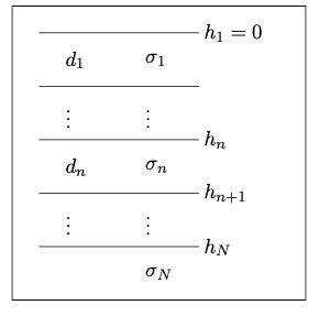
The halfspace is partitioned into \(N\) horizontal, uniform plates of infinite extent. The layer with index \(1\) is the uppermost layer, often referred to as overburden. The layer with index \(N\) (the substratum, sometimes called basement) extends vertically to \(+\infty\). In the case of a uniform halfspace, \(N=1\).

The interfaces between the layers are at \(z=h_n\) where \(1 \le n \le N\). The surface of the conducting Earth is at \(z=h_1 = 0\).

The thickness of layer \(n\) is \(d_n = h_{n+1} - h_n\).

The conductivities are denoted as \(\sigma_n\), \(1 \le n \le N\).

Note that the \(N\)-layered halfspace is composed of \(2N-1\) parameters, i.e., \(N\) conductivities and \(N-1\) thicknesses.

Figure 12.1: The \(N\)-layered halfspace model

We are going to derive expressions for the fields at \(-\infty < z < +\infty\). The resulting expressions will be similar to those derived for the case of a uniform halfspace.

We take the following steps to solve the problem:

First, we formulate a boundary value problem for the potential inside the layer with index \(n\), \(1 \le n \le N\), and extend its solution upwards to the layer denoted \(n-1\) by applying appropriate conditions of continuity of the fields and the potential.

In what follows, we only consider that part of the solution of the Helmholtz equation depending on \(z\), i.e., \(V(z, \lambda)\).

Inside the layer with index \(n\) we define the function \(\lambda_n = \lambda_n(\lambda) = \sqrt{\lambda^2 + i\omega\mu_0 \sigma_n}\).

We assume that there are both upward and downward travelling waves arising from reflections at the discontinuities (jumps) of the electrical conductivity between adjacent uniform layers.

Let the function \[ \begin{equation} \begin{aligned} V(z, \lambda) &=\gamma_{n}^{-}(\lambda) e^{-\lambda_{n}\left(z-h_{n}\right)}+\gamma_{n}^{+}(\lambda) e^{+\lambda_{n}\left(z-h_{n}\right)} \\ &=\gamma_{n}^{-}\left[e^{-\lambda_{n}\left(z-h_{n}\right)}+ \textcolor{red}{r_{n}} e^{+\lambda_{n}\left(z-h_{n}\right)}\right] \end{aligned} \end{equation} \] be the solution to the Helmholtz equation \[ \begin{equation} V''(z) = \lambda_n^2 V(z) \end{equation} \] for \(h_n < z < h_{n+1}\).

Note that \(\textcolor{red}{r_n} := \dfrac{\gamma_n^+}{\gamma_n^-}\) is the ratio of the amplitudes of upward (reflected) and downward (transmitted) travelling waves at the interface at \(z=h_n\).

Note

If the magnetic permeability is non-uniform with depth, i.e., \(\mu = \mu(z)\), then we may replace \(\lambda_n\) by \(\eta_n = \sqrt{\lambda^2 + i\omega\mu_n \sigma_n}/ \mu_n\).

12.2 Recursion

Let’s first analyze the wave propagation in the infinite layer \(N\).

There only exists a downward propagating (outgoing) wave with \[ \begin{equation} V(z, \lambda)=\gamma_{N}^{-}(\lambda) e^{-\lambda_{N}\left(z-h_{N}\right)}, \qquad z \gt h_{N}. \end{equation} \] This is in complete agreement with the uniform case, where \(N=1\), \(h_N = 0\), and therefore \(\gamma_{N}^{-}(\lambda) = \gamma^{-}(\lambda)\).

The important question is:

How does a jump of conductivity \(\sigma_{n+1} - \sigma_n \ne 0\) in the plane \(z=h_{n+1}\) affect the propagation of the partial waves \(V(z, \lambda)\)?

To answer this question, knowledge about the behaviour of field components (or the potential) is required.

We already know that the potential and its vertical derivative are continuous in \(z=0\). In the case of a layered halfspace, this can be extended to any plane \(z=h_n\), \(1 \le n \le N\).

The continuity still holds for the function \[ \begin{equation} B(z, \lambda)=-\frac{V^{\prime}(z, \lambda)}{V(z, \lambda)} \end{equation} \] i.e., the assumption of continuity is also valid for the ratio of the two continuous functions \(V^\prime\) and \(V\) for any value of \(\lambda\).

Of particular interest is the evaluation of \(B(z)\) at the interface between two adjacent layers.

To this end, we define the interface admittance \(B_n\) of the wave by setting \[ \begin{equation} B_{n}:=B\left(h_{n}\right)=-\frac{V^{\prime}\left(h_{n}\right)}{V\left(h_{n}\right)} \end{equation} \]

For EM applications operating on and above the Earth’s surface, the surface admittance \(B_1\) evaluated in \(z=h_1 = 0\) is most important.

Later we will introduce the surface impedance \(Z_1\), with the help of which we infer other quantities such as the apparent resistivity and phase.

Summary

• We have formulated an ansatz for \(V(z)\) in any layer
• This ansatz can be interpreted as the linear combination of upward and downward propagating partial waves with exponential decay inside the layer and fixed interface amplitudes at the adjacent interfaces
• The two coefficient functions \(\gamma_n^+\) and \(\gamma_n^-\) for the \(n\)-th layer are still to be determined
• To this end, we enforce conditions of continuity at those interfaces

In the following we introduce auxiliary functions like the reflection coefficient function \(r_n(\lambda)\).

12.2.1 Behaviour of \(V(z)\) in layer \(N\)

With \(r_n\) we describe the ratio of upward and downward travelling partial waves.

In \(z=h_N\) we don’t observe an upward travelling wave, i.e., there is no reflection arising from an interface below \(z=h_N\).

Therefore, \(r_N(\lambda) = 0\) in \(z=h_N\) for all \(\lambda\).

The layer \(N\), also called the substratum, acts like a homogeneous halfspace.

12.3 Implementation

In the following we derive the computation of \(B_1\) using sympy.

First, we define a few symbolic variables.

• λₙ: wave number in layer \(n\)
• γ⁻, γ⁺: coefficient functions in layer \(n\)
• Bₙ₊₁: admittance evaluated at \(z=h_{n+1}\)
• rₙ: reflection coefficient at \(z=h_n\)
• dₙ: thickness of layer \(n\)
• hₙ: \(z\)-coordinate at the top of layer \(n\)

z, r_n, d_n = symbols("z r_n d_n", real=True)
h_n = symbols("h_n", real=True, positive=True)
lambda_n, B_np1, gamma_minus, gamma_plus = symbols("lambda_n B_{n+1} gamma^- gamma^+")

Further, we define V(z) as a symbolic expression for \(V(z)\):

V = lambda z: gamma_minus * (exp(-lambda_n * (z - h_n)) + r_n * exp(lambda_n * (z - h_n)))
print_latex('V(z) =')
V(z)

\(V(z) =\)

\(\displaystyle \gamma^{-} \left(r_{n} e^{\lambda_{n} \left(- h_{n} + z\right)} + e^{- \lambda_{n} \left(- h_{n} + z\right)}\right)\)

B(z) is the implementation of the admittance function \(B(z)\):

B = lambda z: -diff(V(z), z) / V(z)
print_latex('B(z) = ')
B(z).simplify()

\(B(z) = \)

\(\displaystyle \frac{\lambda_{n} \left(- r_{n} + e^{2 \lambda_{n} \left(h_{n} - z\right)}\right)}{r_{n} + e^{2 \lambda_{n} \left(h_{n} - z\right)}}\)

B_n is the interface admittance at the top of layer \(n\):

B_n = B(z).subs(z, h_n).simplify()
print_latex("B_n = ")
B_n

\(B_n = \)

\(\displaystyle \frac{\lambda_{n} \left(1 - r_{n}\right)}{r_{n} + 1}\)

We observe that \[ \begin{equation} B_{n}=\lambda_{n} \frac{1-r_{n}}{1+r_{n}}. \end{equation} \tag{12.1}\] We now have a representation of the interface admittance in terms of the layer properties \(\lambda_n\) and the reflection coefficient \(r_n\).

However, the \(r_n\) remains undetermined. We try to eliminate \(r_n\) from the equation above.

To this end, we express \(B(z)\) at \(z=h_{n+1}\) using the layer thickness \(d_n\).

B(z).subs(z - h_n, d_n).simplify()

\(\displaystyle \frac{\lambda_{n} \left(- r_{n} e^{2 d_{n} \lambda_{n}} + 1\right)}{r_{n} e^{2 d_{n} \lambda_{n}} + 1}\)

We rewrite the result and obtain \[ \begin{equation} B_{n+1}=\lambda_{n} \frac{1-r_{n} e^{2 \lambda_{n} d_{n}}}{1+r_{n} e^{2 \lambda_{n} d_{n}}}. \end{equation} \]

Now we have found a second equation which contains \(r_n\), which we eliminate in the following step.

We rearrange the equation and bring \(r_n\) to the left.

With the help of sympy we carry out the following steps:

• Evaluate \(B(z)\) in \(z=h_{n+1}\) by
• Substitute (subs) \(h_{n+1} - h_n\) by \(d_n\)
• Solve (solve) the equation for \(r_n\)
• Save the result as r in sympy

Thus, we have found an expression which introduces a link to the layer \(n+1\), and enables us to eliminate \(r_n\).

r = solve(B(z).subs(z - h_n, d_n) - B_np1, r_n)
display(HTML("\\(r_n = \\)"))
r[0]

\(r_n = \)

\(\displaystyle \frac{\left(- B_{n+1} + \lambda_{n}\right) e^{- 2 d_{n} \lambda_{n}}}{B_{n+1} + \lambda_{n}}\)

Given this intermediate result, we are now prepared to substitute the expression \(r_n\) in equation 12.1.

We have obtained an important, yet unfinished, intermediate result, which already contains a recursion \[ B_n \leftarrow B_{n+1} \qquad\text{for } n= N-1, N-2, \dots, 1. \]

display(HTML("\\( B_n = \\)"))
B_n.subs(r_n, r[0]).simplify().simplify()

\( B_n = \)

\(\displaystyle \frac{\lambda_{n} \left(B_{n+1} - \lambda_{n} + \left(B_{n+1} + \lambda_{n}\right) e^{2 d_{n} \lambda_{n}}\right)}{- B_{n+1} + \lambda_{n} + \left(B_{n+1} + \lambda_{n}\right) e^{2 d_{n} \lambda_{n}}}\)

With the following changes we obtain a recursion formula which provides the desired surface admittance \(B_1\):

• Expand with \((\lambda_n + B_{n+1})e^{+\lambda_n d_n}\)
• Collect, sort and factor out \(\lambda_n\) and \(B_{n+1}\) in both numerator and denominator
• Use definitions of hyperbolic functions \(\sinh(z)\) and \(\cosh(z)\)
• Expand with \(1 / \cosh(z)\)

We use \[ \begin{equation} \tanh z=\frac{e^{z}-e^{-z}}{e^{z}+e^{-z}} \end{equation} \] and \[ \begin{equation} {{\cosh z} \atop {\sinh z}} = \frac{1}{2}\left( e^z \pm e^{-z} \right),\qquad z \in \mathbb C, \end{equation} \] and obtain the recursion formula for the admittance at the surface of the Earth:

Wait algorithm for \(\mu_r = 1\)

\[ \begin{equation} \begin{array}{l} \lambda_{n}=\sqrt{\lambda^{2}-k_{n}^{2}}, \qquad n=1,2, \ldots, N \\ B_{N}=\lambda_{N} \\ B_{n}=\lambda_{n} \dfrac{B_{n+1}+\lambda_{n} \tanh \left(\lambda_{n} d_{n}\right)}{\lambda_{n}+B_{n+1} \tanh \left(\lambda_{n} d_{n}\right)}, \qquad n=N-1, \ldots, 1 \end{array} \end{equation} \] This algorithm is known as the Wait algorithm (Wait, J.R., 1954: On the relation between telluric currents and the Earth’s magnetic field, Geophysics, 19, 281-289) PDF

If we let \(\mu_r \ne 1\) in any of the \(N\) layers, we slightly modify the above equations and write

Wait algorithm incorporating \(\mu_r \ne 1\)

\[ \begin{equation} \begin{array}{l} \eta_{n}=\dfrac{\sqrt{\lambda^2 + i\omega\mu_n \sigma_n}}{\mu_n} \qquad n=1,2,\ldots, N \\ \mu_n = \mu_{r,n} \mu_0 \\ B_{N}=\eta_{N} \\ B_{n}=\eta_{n} \dfrac{B_{n+1}+\eta_{n} \tanh \left(\lambda_{n} d_{n}\right)}{\eta_{n}+B_{n+1} \tanh \left(\lambda_{n} d_{n}\right)}, \qquad n=N-1, \ldots, 1. \end{array} \end{equation} \]

Sketch of the fundamental relations for the recursion within the layered halfspace

12.4 Algorithm

We implement the calculation of the admittance as a function called admittance(λ, σ, μ, d, f). The function returns \(B_1\) as a complex-valued number.

The input parameters for an \(n\)-layered halfspace are:

• separation variable \(\lambda\), \(0 \le \lambda < \infty\)
• array of layer conductivities \(\sigma_i\), \(i=1,\dots n\)
• array of layer magnetic permeabilities \(\mu_i = \mu_{ri} \mu_0\), \(i=1,\dots n\)
• array of layer thicknesses \(d_i\), \(i=1,\dots,n-1\)
• frequency in Hz.

def admittance(λ, σ, μ, d, f):
    nl = len(σ)
    ω = 2 * np.pi * f
    α = [np.sqrt(λ**2 + 1j * μ[i] * ω * σ[i]) for i in range(nl)]
    η = [a / m for a, m in zip(α, μ)]
    
    B = np.zeros(nl, dtype=np.complex128)

    B[nl - 1] = η[nl - 1]

    if nl > 1:
        for n in range(nl - 2, -1, -1):
            B[n] = η[n] * \
                    (B[n + 1] + η[n] * np.tanh(α[n] * d[n])) / \
                    (η[n] + B[n + 1] * np.tanh(α[n] * d[n]))

    return B[0]

For \(\lambda = 10\) m\(^{-1}\), \(\sigma=[1, 1]^\top\) S/m, \(\mu=[\mu_0, \mu_0]^\top\) Vs/Am, \(d=1\) m, \(f=1\) Hz we obtain for \(B_1\):

print('B_1 = ')
admittance(10.0, np.array([1, 1]), np.array([1, 1]), np.array([1]), 1.0)

B_1 = 

np.complex128(10.004928726718877+0.31400450112152684j)

We are now able to express the anomalous effect of the layers \(2 \le n \le N\) by the surface admittance \(B_1\).

The resulting admittance formula can be used to simply replace every occurence of \(\lambda_1\) in the equations for the homogeneous halfspace by \(B_1\).

Fields in \(z \le 0\)

\[ \begin{align} E_\varphi & = -\frac{i \omega \mu m}{4 \pi} \left[ \frac{r}{R^3} + \int_0^\infty \frac{\lambda - B_1}{\lambda + B_1}\lambda e^{-\lambda h}e^{\lambda z}J_1(\lambda r)\, \dd\lambda \right] \\ H_r & = \frac{m}{4 \pi} \left[ \frac{3r(z+h)}{R^5} - \int_0^\infty \frac{\lambda - B_1}{\lambda + B_1}\lambda^2 e^{-\lambda h}e^{\lambda z}J_1(\lambda r)\, \dd\lambda \right] \\ H_z & = \frac{m}{4 \pi} \left[ \frac{3(z+h)^2 - R^2}{R^5} + \int_0^\infty \frac{\lambda - B_1}{\lambda + B_1}\lambda^2 e^{-\lambda h}e^{\lambda z}J_0(\lambda r)\, \dd\lambda \right] \end{align} \]

Finally, it remains to evaluate the Hankel integrals numerically.

To this end, we need an implementation of a discrete convolution. We use the function convolve:

def convolve(fc, kernel, style="valid"):
    nc = len(fc)
    nu = len(kernel)
    n = nu + nc - 1
    result = np.zeros(n, dtype=type(kernel))
    
    for i in range(nc):
        for j in range(nu):
            result[j + i] += kernel[j] * fc[i]
    
    if style == "full":
        result = result
    elif style == "valid":
        result = result[nc - 1:n - nc + 1]
    
    return result

Here we define the function gethankelfcJ0 that returns the numerical filter coeffients for the function \(J_0(\lambda r)\) fc, the length of the filter nc as well the index which corresponds with the zero position, nc0.

import numpy as np

def gethankelfcJ0():
    fc = np.array([
        +2.898782880000e-07, +3.649351440000e-07, +4.594261260000e-07, +5.783832260000e-07,
        +7.281413380000e-07, +9.166756390000e-07, +1.154026250000e-06, +1.452832980000e-06,
        +1.829008340000e-06, +2.302585110000e-06, +2.898782860000e-06, +3.649351480000e-06,
        +4.594261190000e-06, +5.783832360000e-06, +7.281413220000e-06, +9.166756640000e-06,
        +1.154026210000e-05, +1.452833050000e-05, +1.829008240000e-05, +2.302585270000e-05,
        +2.898782590000e-05, +3.649351860000e-05, +4.594260510000e-05, +5.783833290000e-05,
        +7.281411440000e-05, +9.166758820000e-05, +1.154025730000e-04, +1.452833540000e-04,
        +1.829006940000e-04, +2.302586300000e-04, +2.898778910000e-04, +3.649353620000e-04,
        +4.594249600000e-04, +5.783834370000e-04, +7.281377380000e-04, +9.166748280000e-04,
        +1.154014530000e-03, +1.452825610000e-03, +1.828968260000e-03, +2.302545350000e-03,
        +2.898639790000e-03, +3.649167030000e-03, +4.593733080000e-03, +5.783032380000e-03,
        +7.279414970000e-03, +9.163407050000e-03, +1.153256910000e-02, +1.451458320000e-02,
        +1.826011990000e-02, +2.297010420000e-02, +2.887026190000e-02, +3.626918100000e-02,
        +4.547940310000e-02, +5.694081920000e-02, +7.098730720000e-02, +8.809954260000e-02,
        +1.082238890000e-01, +1.312504830000e-01, +1.550557150000e-01, +1.763715060000e-01,
        +1.856277380000e-01, +1.697780440000e-01, +1.034052450000e-01, -3.025832330000e-02,
        -2.275743930000e-01, -3.621732170000e-01, -2.055004460000e-01, +3.373948730000e-01,
        +3.176898970000e-01, -5.137621600000e-01, +3.091302640000e-01, -1.267575920000e-01,
        +4.619678900000e-02, -1.809686740000e-02, +8.354260500000e-03, -4.473683040000e-03,
        +2.619747830000e-03, -1.601713570000e-03, +9.977178820000e-04, -6.262758150000e-04,
        +3.943388180000e-04, -2.486063540000e-04, +1.568086040000e-04, -9.892662880000e-05,
        +6.241523980000e-05, -3.938053930000e-05, +2.484723580000e-05, -1.567749450000e-05,
        +9.891817410000e-06, -6.241311600000e-06, +3.938000580000e-06, -2.484710180000e-06,
        +1.567746090000e-06, -9.891808960000e-07, +6.241309480000e-07, -3.938000050000e-07,
        +2.484710050000e-07, -1.567746050000e-07, +9.891808880000e-08, -6.241309460000e-08
    ])
    nc = 100
    nc0 = 60
    return fc, nc, nc0

We illustrate the filter coefficients associated with \(J_0(\lambda r)\):

import matplotlib.pyplot as plt
fc0, nc, nc0 = gethankelfcJ0()
fig, ax = plt.subplots(1, 1, figsize=(6,4))
ax.plot([-nc0 + v for v in range(1, nc+1)], fc0)
ax.set_xlabel('index of coefficients')
ax.grid(True)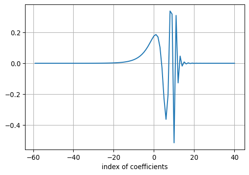

def pos(data):
    """Return positive data; set negative data to NaN."""
    return np.where(data > 0, data, np.nan)

rmin = 10.0
nr = 21
ncnr = nc + nr -1

rr = np.zeros(nr)
R = np.zeros(nr)

z = 0.0
z0 = 0.0
q = 10.0**0.1

mu0 = np.pi * 4e-7

sigma = np.array([0.01])
mu = np.array([1]) * mu0

for n in range(0, nr):
    rr[n] = rmin * q**(n)
    R[n] = np.sqrt(rr[n]**2 + (z - z0)**2)

nf = 61
freq = np.logspace(-1, 5, nf, endpoint=True)
kernel = np.zeros(ncnr, dtype=np.complex128)
Bz = np.zeros((nr, nf), dtype=np.complex128)
Bz0 = (3 * (z - z0)**2 - R**2) / R**5

for k, f in enumerate(freq):
    omega = 2 * np.pi * f
    for nu in range(0, ncnr):
        n = nc0 - nc + nu
        lam = np.exp(-n * 0.1 * np.log(10.0)) / rmin
        B1 = admittance(lam, sigma, mu, [], f)

        E = np.exp(-lam * np.abs(z + z0))

        eta = lam / mu0
        gamma = (B1 - eta) / (B1 + eta) * E
        kernel[nu] = gamma * lam**2


    Bz[:, k] = mu0 / 4 / np.pi * (Bz0 - convolve(fc0, kernel) / rr)

fig, ax = plt.subplots(1, 1, figsize=(6,4))

ax.loglog(freq, pos(np.real(Bz[10, :])) / mu0, color='C0', linestyle='-', label='Re')
ax.loglog(freq, pos(-np.real(Bz[10, :])) / mu0, color='C0', linestyle='--')
ax.loglog(freq, pos(np.imag(Bz[10, :])) / mu0, color='C1', linestyle='-', label='Im')
ax.loglog(freq, pos(-np.imag(Bz[10, :])) / mu0, color='C1', linestyle='--')
ax.grid(True)
ax.legend()
ax.set_xlabel('f in Hz')
ax.set_ylabel(r'$H_z$ in A/m')
ax.set_title(r'$\sigma = $' + str(sigma[0]) + ' S/m, r = ' + '{0:.2f}'.format(rr[10]) + ' m')
ax

Figure 12.2: Vertical magnetic field of a VMD over a uniform halfspace in the frequency domain, calculated using the FHT.

def Hz_analytical(r, f, sigma):
    mu0 = np.pi * 4e-7
    k = np.sqrt(-1j * 2 * np.pi * f * mu0 * sigma)
    B = 9 - (9 + 9 * 1j * k * r - 4 * k**2 * r**2 - 1j * k**3 * r**3) * np.exp(-1j * k * r)
    B = B / (2 * np.pi * k**2 * r**5)
    return B

H = [Hz_analytical(100.0, v, 0.01) for v in freq]

fig, ax = plt.subplots(1, 1, figsize=(6,4))

ax.loglog(freq, pos(np.real(H)) / mu0, color='C0', linestyle='-', label='Re')
ax.loglog(freq, pos(-np.real(H)) / mu0, color='C0', linestyle='--')
ax.loglog(freq, pos(np.imag(H)) / mu0, color='C1', linestyle='-', label='Im')
ax.loglog(freq, pos(-np.imag(H)) / mu0, color='C1', linestyle='--')
ax.grid(True)
ax.legend()
ax.set_xlabel('f in Hz')
ax.set_ylabel(r'$H_z$ in A/m')
ax.set_title(r'$\sigma = $' + str(sigma[0]) + ' S/m, r = ' + '{0:.2f}'.format(rr[10]) + ' m')
ax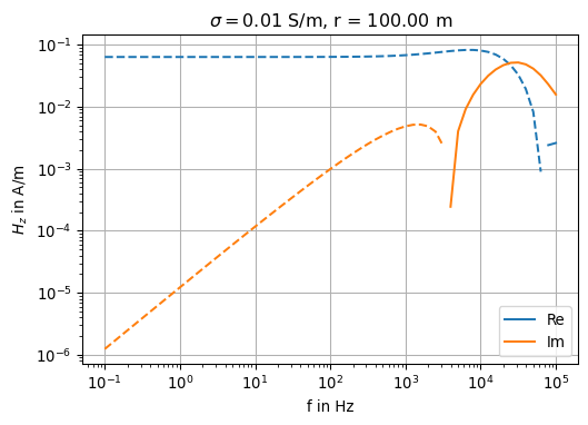

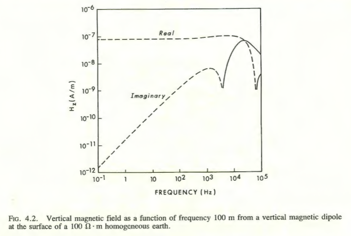
Figure 12.3: Vertical magnetic field of a VMD over a uniform halfspace in the frequency domain, calculated using an analytical formula.

Figure 12.4: Reference to Fig. above above taken from Ward & Hohmann (1988)

As we can see from visual inspection of all three illustrations given above, the Fast Hankel Transform approach works well.

12.5 Application: Airborne EM

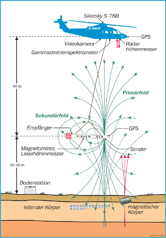
The Federal Institute for Geosciences and Natural Resources (BGR Hannover) operates the 5-frequency EM induction system DIGHEM (Fugro Airborne Survey, Canada). It employs an HCP configuration, hence our example using the VMD is well suited.

The 5 frequencies used by the DIGHEM system are between \(10^{2}\) and \(10^{5}\) Hz. The distance between transmitter and receilver coils are 8 m. The instrument is contained in a tube (bird), which is towed by a 45 m long cable about 30-40 m above ground.

Sketch of the BGR airborne geophysical system, Source: BGR (www.bgr.bund.de)

freq = np.array([387, 1820, 8225, 41550, 133200])
nf = 5
r = 8.0
z = -30.0
z0 = -30.0

To assess the validity of our code, we choose as reference the published 4-layer repsonse from Siemon et al. (2009), Table 1:

rho = np.array([200, 100, 5, 1000])
thk = np.array([20, 30, 10])
sigma = 1.0 / rho
mu = np.ones(len(rho)) * mu0

rmin = r
nr = 1
ncnr = nc + nr - 1

rr = np.zeros(nr)
R = np.zeros(nr)

for n in range(0, nr):
    rr[n] = rmin * q**(n)
    R[n] = np.sqrt(rr[n]**2 + (z - z0)**2)

kernel = np.zeros(ncnr, dtype=np.complex128)
Bz = np.zeros((nr, nf), dtype=np.complex128)
Bz0 = (3 * (z - z0)**2 - R**2) / R**5

for k, f in enumerate(freq):
    omega = 2 * np.pi * f
    for nu in range(0, ncnr):
        n = nc0 - nc + nu
        lam = np.exp(-n * 0.1 * np.log(10.0)) / rmin
        B1 = admittance(lam, sigma, mu, thk, f)

        E = np.exp(-lam * np.abs(z + z0))

        eta = lam / mu0
        gamma = (B1 - eta) / (B1 + eta) * E
        kernel[nu] = gamma * lam**2


    Bz[:, k] = mu0 / 4 / np.pi * (Bz0 - convolve(fc0, kernel) / rr)

The quantity relevant to the airborne EM data interpretation is the normalized secondary field \[ \begin{equation} \begin{split} R & = \Re \left(\frac{B_z}{B_z^{air}} - 1 \right) \\ Q & = \Im \left(\frac{B_z}{B_z^{air}}\right). \end{split} \end{equation} \]

Those quantities R (for real part) and Q (for quadrature part) are usually given in units of ppm.

Z = Bz / (mu0 * Bz0 / 4 / np.pi)
R_ppm = 1e6 * (np.real(Z) - 1)
Q_ppm = 1e6 * np.imag(Z)

The reference data from Siemon et al. is

R_BGR = np.array([21.8, 129.1, 280.4, 734.7, 1506])
Q_BGR = np.array([68.36, 164.4, 291.5, 747.4, 1047])

fig, ax = plt.subplots(1, 1, figsize=(6,4))
ax.loglog(freq, R_ppm.ravel(), marker='o', label="R FHT FG")
ax.loglog(freq, R_BGR.ravel(), marker='o', label="R FHT BGR")
ax.loglog(freq, Q_ppm.ravel(), marker='o', label="Q FHT FG")
ax.loglog(freq, Q_BGR.ravel(), marker='o', label="Q FHT BGR")
ax.legend()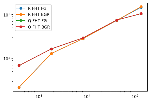

12.6 Summary

We have learned that field values can be computed very accurately and efficiently using the digital filter method.

The numerical effort lies in providing a (large) number of evaluations of the kernel function \(f\) at given points \(\lambda\).

In a similar manner, the inverse Fourier transform from the frequency domain to the time domain can be implemented.

Corresponding filter coefficients also exist for \(J_{-1/2}\) and \(J_{+1/2}\).

Note

It remains to be said, that the numerical evaluation of the convolution is an expensive bottleneck, when the fields have to be computed at different \(z\) levels.

Ward, S.H. & Hohmann, G.W., 1988. Electromagnetic theory for geophysical applications. Electromagnetic methods in applied geophysics, Vol. 1, pp. 131–311.