We associate both sets of fields 2.1 and 2.2 by a Fourier transform: \[
\begin{align}
F(\omega) & = \int\limits_{-\infty}^\infty f(t) e^{-i\omega t}\,\mathrm d t
\end{align}
\tag{3.1}\]
Here \(\omega = 2 \pi f\) is the angular frequency.
Warning
Note that there exist different definitions of the above transform pair. For a detailed overview see this Wikipedia page.
We use a positive exponent in the time-dependency expressed by \(\exp(+i \omega t)\).
Also note that the normalizing factor \(\frac{1}{2 \pi}\) appears in the synthesis.
The Fourier transform can also be used to transform a function of spatial variables into the wave number domain. In this case, we replace \(\omega\) with \(k\) and the time \(t\) with, e.g., \(x\).
The first equation 3.1 is called harmonic analysis, whereas the second equation 3.2 is called harmonic synthesis.
Note
In the following, we most often make use of the synthesis to construct field components from their spectral content, the partial or plane waves.
To put it in simple words, we try to combine simple things to create complex things. More precisely, we add many sine and cosine wave harmonics to approximate a function in space or time.
3.1 Example
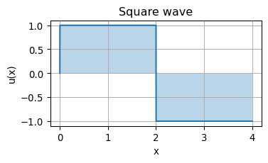
In this example we use a Fourier series expansion to approximate the periodic square function\(u(x)\) of length \(2L\).
An analytic formula for a square wave with unit amplitude and period \(2L\) is given by \(u(x) = \mathrm{sign}(\sin(\frac{\pi x}{L})\).
Show the code
x = np.arange(0, 4, 0.001)u = [np.sign(np.sin(np.pi * v /2)) for v in x]fig, ax = plt.subplots(figsize=(4, 3))ax.plot(x, u)ax.fill_between(x, u, np.zeros_like(u), alpha=0.3)ax.set_xlabel('x')ax.set_ylabel('u(x)')ax.set_title('Square wave')ax.set_aspect('equal')ax.grid(True)
The Fourier series expansion for a periodic square wave \(u(x)\) is
This function is called uk and takes the arguments x and the index k. The window length L takes the default setting of 0.5.
Show the code
def uk(x, k, L=0.5):return np.sin(np.pi * (2* k -1) * x / L) / (2* k -1)
Next, we implement the summation over all \(k\) sine terms, i.e., \[
u(x) \approx \frac{4}{\pi} \sum_{k=1}^N u_k(x)
\]
Show the code
def u(x, k, L): value =4/ np.pi *\sum(uk(x, i, L) for i inrange(1, k+1)) if k >0else np.zeros_like(x)return value
Show the code
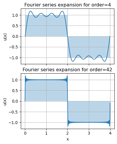
L =2order =4x = np.arange(0, 2*L, 0.001)u_n = [np.sign(np.sin(np.pi * v / L)) for v in x]fig, ax = plt.subplots(nrows=2, ncols=1, sharex=True, layout='constrained')ax[0].plot(x, u(x, order, L))ax[0].fill_between(x, u_n, np.zeros_like(u_n), alpha=0.3)#ax[0].set_xlabel('x')ax[0].set_ylabel('u(x)')ax[0].set_title(f'Fourier series expansion for order={order}')ax[0].set_aspect('equal')ax[0].grid(True)order =42ax[1].plot(x, u(x, order, L))ax[1].fill_between(x, u_n, np.zeros_like(u_n), alpha=0.3)ax[1].set_xlabel('x')ax[1].set_ylabel('u(x)')ax[1].set_title(f'Fourier series expansion for order={order}')ax[1].set_aspect('equal')ax[1].grid(True);
Note
Note the Gibbs phenomenon at the jumps of the square wave. This is a typical behaviour of a piecewise differentiable continuous periodic function. As the expansion order gets large, the overshoot does not die out, but approaches a finite limit.
It can be shown that, for sufficiently large \(N\), the full overshooting is around 17.9 % larger than the jump in the original function.